4.2.1. Example 1

4.2.1.1. Thermal expansion of a beam

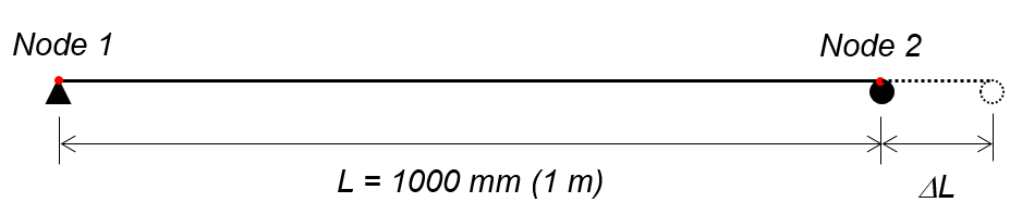
Elevation of beam

Example Overview: A steel beam is heated to 1180 ^o C. Horizontal displacement of right end is recorded. This displacement is normalized against the original length and plotted against temperature. The calculated thermal expansion is compared against the steel temperature-dependent thermal expansion in Eurocode 3, Part 1-2 [1].

Download Example 1 files:

Example1.tcl.

Example 1 Outputs.

4.2.1.1.1. Material Properties

The uniaxialMaterial Steel01Thermal includes temperature-dependent steel thermal and mechanical properties per Eurocode 3 [1]. More details of Steel01 can be found at: Steel01 Material

uniaxialMaterial Steel01Thermal $matTag $Fy $Es $b;

Es = 210 GPa (Young’s modulus of elasticity at ambient temperatures)

Fy = 250 MPa (Yield strength of material at ambient temperatures)

b = 0.001 (Strain-Hardening Ratio)

4.2.1.1.2. Transformation

The beam is expanding in one direction, therefore, 2nd order bending effects do not need to be considered.

geomTransf Linear $transftag;

Learn more about geometric transofrmations: Geometric Transformation

4.2.1.1.3. Section

The discretization of the steel section into four fibers is shown using the code below:

section FiberThermal secTag -GJ $Es{

set numSubdivIJ 2;     # horizontal

set numSubdivJK 2;     # vertical

set yI -100; #mm

set zI -200; #mm

set yJ 100; #mm

set zJ -200; #mm

set yK 100; #mm

set zK 200; #mm

set yL -100; #mm

set zL 200; #mm

patch quad $matTag $numSubdivIJ $numSubdivJK $yI $zI $yJ $zJ $yK $zK $yL $zL

Sections that will be subjected to thermal loading must be created with fiberThermal or fibersecThermal.

In previous versions of OpenSees, a default value for torsional stiffness was used (GJ). In versions 3.1.0 and newer fiber sections require a value for torsional stiffness. This is a 2D example with negligible torsion, however a value is required. The Young’s Modulus is used for convenience.

The discretization can be visualized as such:

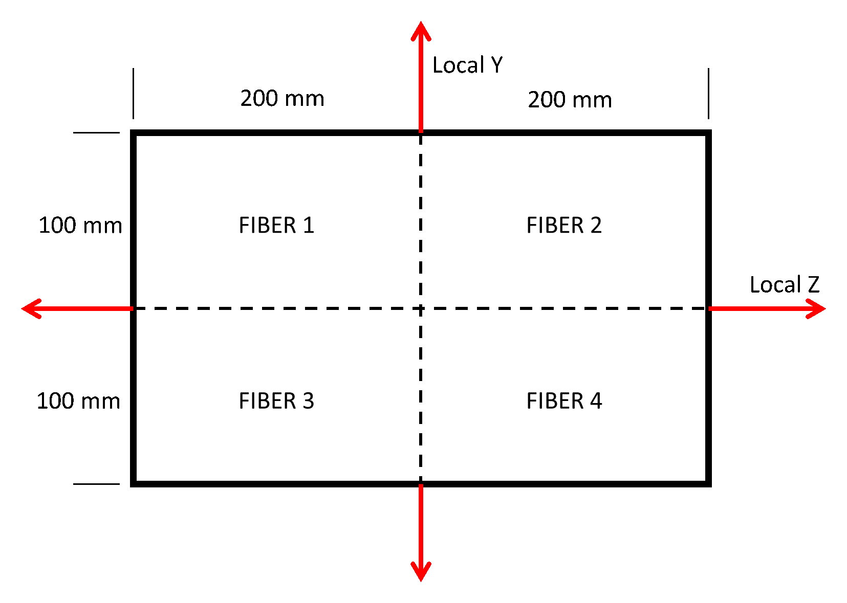
Cross section of rectangular beam showing fiber discretization

4.2.1.1.4. Elements

dispBeamColumnThermal elements are used because temperature-dependent thermal and mechanical steel properties can be applied to these elements. Any portion of the structure that is being heated must use elements that are compatible with uniaxialMaterial Steel01Thermal. At the time this model was developed, dispBeamColumnThermal was the only element type that could have tempurature-dependent thermal and mechanical properties applied to them.

The beam is made of one element with 5 iteration points and connects nodes 1 & 2. OpenSees is sensitive to the number of iteration points in each element and this could change the result of the recorded displacement. For this reason, it is important to perform these benchmarking examples to establish how many iteration points allows for convergence to the expected recorded displacement. To code the number of iteration points, we use the following syntax:

dispBeamColumnThermal eleTag iNode jNode numIntgrPts secTag TransfTag;

element dispBeamColumnThermal 1 1 2 5 $secTag $transftag;

4.2.1.1.5. Output Recorders

Displacement of the end node (2) in DOF 1 (Horizontal Displacement) is what we want to record. To do so, a folder within your working directory must be created. $dataDir is the command to create that folder and should be defined at the beginning of the model. This is where your output files will be saved.

set dataDir Examples/EXAMPLE2_OUTPUT;

file mkdir $dataDir;

recorder Node -file $dataDir/Node2disp.out -time -node 2 -dof 1 disp;

Learn more about the Recorder Command: ` Recorder Command <http://opensees.berkeley.edu/wiki/index.php/Recorder_Command>` __

4.2.1.1.6. Thermal Loading

This particular model is heating a beam to a set temperature over the time period of the model. We are not asking OpenSees to use a specific time-temperature curve, rather linearly ramp up the temperature from ambient to 1180 ^o C.

Therefore, we set the maximum temperature as follows:

T = Max Tempurature [deg celcius]

set T 1180;

In OpenSees, the user can define 2 or 9 temperature data points through the cross section. In a 2D analysis framework, like this example, temperature data point locations are specified on the y-axis of the local coordinate system (as shown in the figure below), and are linearly interpolated between the defined points. Because this example is using a uniformly heated beam, the entire cross section is one temperature, and two temperature points on each extreme fiber on the y-axis will be chosen. The beam has a depth of 400 mm, therefore, Y1 = 200 mm & Y2 = -200 mm for the top and bottom fibers respectively.

Location of bottom extreme fiber of beam [mm]

set Y1 100;

Location of top extreme fiber of beam [mm]

set Y2 -100;

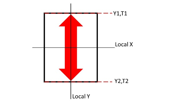
Location of defined input temperature locations on the member cross section

The bottom extreme fiber temperature must be defined first. The target maximum temperature for each extreme fiber is set to 1180^oC and will be increased incrementally and linearly as the time step continues in the analysis. An external temperature data set could also be used for more complex temperature loading. The syntax for this is:

Thermal loading pattern

pattern Plain 1 Linear { eleLoad -ele 1 -type -beamThermal $T $Y2 $T $Y1 };

4.2.1.1.7. Thermal Analysis

Thermal loading is applied in 1000 steps, with a load factor of 0.001. Each step is a 0.001 increment of the maximum temperature specified in the thermal loading step: $T. The analysis is a static analysis and the contraints of the beam are plain. 1000 increments was also used during thermal analysis to allow for easy correlation between the input temperatures and the recorded output.

A variety of load factors were examined and the solution converged when a load factor of 0.001 was used. OpenSees is sensitive to the load factor, therefore, it is important to ensure that benchmarking examples are performed to determine the proper load factor to use in structural fire engineering analyses.

set Nsteps 1000

set Factor [expr 1.0/$Nsteps];

integrator LoadControl $Factor;

analyze $Nsteps;

4.2.1.1.8. Output Plots

After the model has completed running, the results will be a horizontal displacement of the right end of the beam. Since the temperature was linearly ramped up from ambient to 1180 ^o C, the user can develop a temperature history that matches every increment of the model.

Thermal expansion is the change is length divided by the original length. This could also be called thermal strain. The thermal expansion of the beam is plotted below and compared to the Eurocode 3 [1]temperature-dependent thermal expansion. We can see that the modeled thermal expansion matches the material properties. This is important to check that the temperatures and material properties are assigned propertly in the model.

Thermal expansion of the beam recorded at node 2

4.2.1.1.9. Sources

[1] European Committee for Standardization (CEN). (2005). Eurocode 3: Design of Steel Structures, Part 1.2: General Rules - Structural Fire Design.