4.2.5. Example 5
4.2.5.1. A two-bay frame that measures 2.4 m x 1.18 m with a 60 N/m distributed load and column point loads is subjected to a fire in one of the bays. The heated bay is heated linearly to a target temperature of 550 o C.
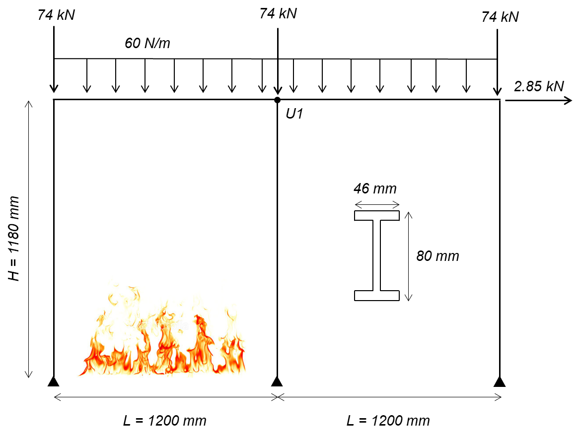
Elevation of two-bay frame
Example overview: This example will combine the modeling methodologies developed through the other examples and apply them to a two-bay frame with a fire in one of the bays. Recorded data from the OpenSees analysis will be compared with the experimental test data [2]. Heat transfer analyses were performed using a commercially available finite element program to calculate the temperature distribution through the cross sections when the members are exposed to a linear gas time-temperature curve. Horizontal displacement of upper corners, U1 & U2 are recorded.
Download Example 5 files:
4.2.5.1.1. Objectives
Example 5 Objectives: 1. Create a two-bay frame in OpenSees using displacement-based elements with tempurature-dependent material properties, 2. Implementing user-defined time-tempurature histories for the elements calculated through heat transfer analysis, and 3. Compare recorded parameters from the OpenSees model to experimental testing data [2] to benchmark modeling methodologies.
Experimental Test Overview
A two-bay frame was tested by researchers [2]. Each bay size was 1.2 m in width and 1.18 m in height. Point loads were applied at the beam-column joints in the lateral and gravity directions in addition to a uniformly distributed load applied to the beams. The columns and beam of one of the bays was heated using electrical heaters that surrounded each of the members, therefore, uniformly heating each member (there was no thermal gradient through the cross section). The temperature was increased until failure.
4.2.5.1.2. Material
The uniaxialMaterial Steel01Thermal includes temperature-dependent steel thermal and mechanical properties per Eurocode 3 [1]. More details of Steel01 can be found at: Steel01 Material
Es = 210 GPa (Young’s modulus of elasticity at ambient temperatures)
Fy = 355 MPa (Yield strength of material at ambient temperatures)
b = 0.001 (Strain-Hardening Ratio)
- set matTag 1;
- uniaxialMaterial Steel01Thermal $matTag $Fy $Es $b;
4.2.5.1.3. Transformation
Because the beams and columns in this example experience bending, 2nd order bending effects were considered using the Corotational geometric transformation.
- geomTransf Corotational $transftag;
Learn more about geometric transofrmations: Geometric Transformation
4.2.5.1.4. Section
This example uses an external .tcl script to define the cross section. This script uses fibersecThermal to procure a fibered W-shape section with a section tag to be used while defining elements. Eight fibers are used throughout the web and four fibers within each flange.
In previous versions of OpenSees, a default value for torsional stiffness was used (GJ). In versions 3.1.0 and newer fiber sections require a value for torsional stiffness. This is a 2D example with negligible torsion, however a value is required. The Young’s Modulus is used for convenience. Wsection dimensions are (units are meters):
- set secTag 1; # section Tag
set d 0.08; # depth of beam set bf 0.046; # flange width set tf 0.0052; # flange thickness set tw 0.0038; # web thickness
secTag - section tag
matTag - material tag
d = nominal depth
tw = web thickness
bf = flange width
tf = flange thickness
nfdw = number of fibers along web depth
nftw = number of fibers along web thickness
nfbf = number of fibers along flange width
nftf = number of fibers along flange thickness
Gj = torsional stiffness
WsectionThermal secTag matTag d bf tf tw nfdw nftw nfbf nftf Gj
- WsectionThermal $secTag $matTag $d $bf $tf $tw 8 1 1 4 $Es

Cross section of W-shape showing fibers in the flanges and the web
4.2.5.1.5. Element
dispBeamColumnThermal elements are used because temperature-dependent thermal and mechanical steel properties can be applied to these elements. Any portion of the structure that is being heated must use elements that are compatible with uniaxialMaterial Steel01Thermal. At the time this model was developed, dispBeamColumnThermal was the only element type that could have tempurature-dependent thermal and mechanical properties applied to them.
dispBeamColumnThermal $eleTag $iNode $jNode $numIntgrPts $secTag $TransfTag;
- element dispBeamColumnThermal 1 1 2 3 $secTag $transftag;
Each column and beam element is created using ten displacement-based elements with 3 iteration points in each element.
4.2.5.1.6. Output Recorders
$dataDir is defined at the beginning of the model, this creates a folder within your working directory where output files will be saved.
- set dataDir Examples/EXAMPLE5_OUTPUT;
- file mkdir $dataDir;
displacements of node U1 (node 11, top left), DOF 1 (Horizontal Displacement)
- recorder Node -file $dataDir/Midspan_BeamDisp.out -time -node 11 -dof 1 disp;
displacements of node U2 (node 22, top-middle), DOF 1 (Horizontal Displacement)
- recorder Node -file $dataDir/Midspan_BeamDisp.out -time -node 22 -dof 1 disp;
Reaction forces at support nodes (1, 12 & 23):
- recorder Node -file $dataDir/RXNS.out -time -node 1 12 23 -dof 2 3 reaction;
Learn more about the Recorder Command: Recorder Command
4.2.5.1.7. Thermal Loading
In this model, the beams and columns of the left bay are heated by increasing the temperature linearly from ambient temperature until failure. The right bay remains at ambient tempurature.
Therefore, we set the maximum temperature as follows:
T = Max Temperature [ o C]
- set T 550;
In OpenSees, the user can define 2 or 9 temperature data points through the cross section. In a 2D analysis framework, like this example, temperature data point locations are specified on the y-axis of the local coordinate system (as shown in the figure above). And are linearly interpolated between the defined points. Because this example is using a uniformly heated beam, two temperature points on each extreme fiber on the y-axis will be chosen. The beam has a depth of $d, therefore, Y1 = $d/2 & Y2 = -$d/2 the top and bottom fibers respectively.
Top fiber of beam
- set Y1 [expr $d/2];
Bottom fiber of beam
- set Y2 [expr -$d/2];
Location of defined input temperature locations on the member cross section (both beam and columns)
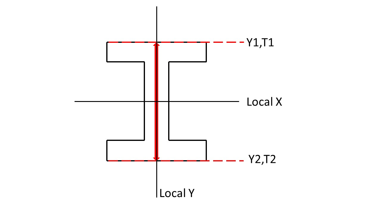
The bottom extreme fiber temperature must be defined first. The target maximum temperature for each extreme fiber is set to 550 o C and will be increased linearly and incrementally as the time step continues in the analysis. An external temperature data set can could also be used for more complex temperature loading.
Using a for-loop and a plain linear loading pattern, elements 1-20 & 31-40 will be subjected to tempurature, $T. These elements define the heated bay.
- pattern Plain 2 Linear {
- for {set i 1} {$i <= 20} {incr i} { eleLoad -ele $i -type -beamThermal $T $Y2 $T $Y1;}
- for {set i 31} {$i <= 40} {incr i} {eleLoad -ele $i -type -beamThermal $T $Y2 $T $Y1;}};
4.2.5.1.8. Thermal Analysis
Thermal loading is applied in 1000 steps, with a load factor of 0.001. Each step is a 0.001 increment of the maximum temperature specified in the thermal loading step: $T. The analysis is a static analysis and the contraints of the beam are plain. 1000 increments was also used during thermal analysis to allow for easy correlation between the input temperatures and the recorded output. Each step is an 0.001 increment of the maximum temperature specified in the thermal loading step: `T.
A variety of load factors were examined and the solution converged when a load factor of 0.001 was used. OpenSees is sensitive to the load factor, therefore, it is important to ensure that benchmarking examples are performed to determine the proper load factor to use in structural fire engineering analyses.
- set Nstep 1000
- set Factor [expr 1.0/$Nstep];
- integrator LoadControl $Factor;
- analyze $Nstep;
4.2.5.1.9. Output Plots
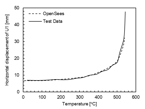
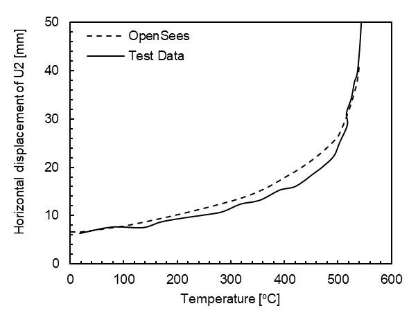
After the model has completed running, the results will be horizontal displacments of the recorded node. Since the temperature was linearly ramped up from ambient to 550 o C, the user can develop a temperature history that matches every increment of the model. The displacements are benchmarked against test data [2] as shown in the figure below.
Node U1 horizontal displacement versus temperature compared with the testing data
Node U2 horizontal displacement versus temperature compared with the testing data
4.2.5.1.10. Sources
[1] European Committee for Standardization (CEN). (2005). Eurocode 3: Design of Steel Structures, Part 1.2: General Rules - Structural Fire Design.
[2] Rubert A, Schaumann P. (1986). “Structural steel and plane frame assemblies under fire action.” Fire Safety Journal, vol. 10, pp.173–184.