3.2.11. responseSpectrumAnalysis Command
- responseSpectrumAnalysis $tsTag $direction <-scale $scale> <-mode $mode>
- responseSpectrumAnalysis $direction -Tn $Tn -Sa $Sa <-scale $scale> <-mode $mode>
Argument |
Type |
Description |
|---|---|---|
$tsTag |
integer |
The tag of a previously defined Time Series Command. This list stores the Tn and Sa values. If you want to use the timeSeries, you cannot specify the -Tn and -Sa options |
-Tn |
string |
Tells the command to use the $Tn list, instead of the timeSeries, to get the periods of the response spectrum function |
$Tn |
list float |
The list of periods of the response spectrum function |
-Sa |
string |
Tells the command to use the $Sa list, instead of the timeSeries, to get the accelerations of the response spectrum function |
$Sa |
list float |
The list of accelerations of the response spectrum function |
$direction |
integer |
The 1-based index of the excited DOF (1 to 3 for 2D problems, or 1 to 6 for 3D problems). |
-scale |
string |
Tells the command to use a user-defined scale factor for the computed modal displacements. Not used, placeholder for future implementation. |
$scale |
float |
User-defined scale factor for the computed modal displacements. Not used, placeholder for future implementation. |
-mode |
string |
Tells the command to compute the modal displacements for just 1 specified mode (by default all modes are processed). |
$mode |
integer |
The 1-based index of the unique mode to process. |
Note
This command can be used only if a previous call to eigen Command and modalProperties Command has been performed.
It computes only the modal displacements, any modal combination is up to the user.
The scale factor (-scale $scale) for the output modal displacements is not used now, and it’s there for future implementations. When your model is linear elastic there is no need to use this option. It will be useful in future when we will allow using this command on a nonlinear model as a linear perturbation about a certain nonlinear state. In that case, the scale factor can be set to a very small number, so that the computed modal displacements will be very small (linear perturbation) and will not alter the nonlinear state of your model. Then the inverse of the scale factor can be used to post-multiply any result for post-processing.
3.2.11.1. Theory
\(\lambda_i\) is the eigenvalue
\(\Phi_{ij}^n\) is the eigenvector
\(MPF_{ij}\) is the modal participation factor
\(RSf\left(T_i\right)\) is the response spectrum function value at period \(T_i\)
and \(T_i\) is the period \(\frac{2\pi}{\sqrt{\lambda_i}}\)
Example 1: Simple call
The following example shows how to call the responseSpectrumAnalysis command for all modes, using the time series 1 (or lists Tn and Sa) along the DOF 1 (Ux)
Tcl Code using timeSeries
set tsTag 1; # use the timeSeries 1 as response spectrum function
set direction 1; # excited DOF = Ux
responseSpectrumAnalysis $tsTag $direction
Tcl Code using lists
set Tn {0.0 0.1 0.4 .... }; # the periods
set Sa {1.9 3.7 4.9 .... }; # the accelerations
set direction 1; # excited DOF = Ux
responseSpectrumAnalysis $direction -Tn $Tn -Sa $Sa
Tcl Code using expanded lists
set Tn {0.0 0.1 0.4 .... }; # the periods
set Sa {1.9 3.7 4.9 .... }; # the accelerations
set direction 1; # excited DOF = Ux
responseSpectrumAnalysis $direction -Tn {*}$Tn -Sa {*}$Sa
Python Code using timeSeries
tsTag = 1 # use the timeSeries 1 as response spectrum function
direction = 1 # excited DOF = Ux
responseSpectrumAnalysis(tsTag, direction)
Python Code using lists
Tn = [0.0 0.1 0.4 .... ] # the periods
Sa = [1.9 3.7 4.9 .... ] # the accelerations
responseSpectrumAnalysis(direction, '-Tn', *Tn, '-Sa', *Sa)
Example 2: Iterative call
The following example shows how to call the responseSpectrumAnalysis command for 1 mode at a time, using the time series 1 along the DOF 1 (Ux)
Tcl Code
set tsTag 1; # use the timeSeries 1 as response spectrum function
set direction 1; # excited DOF = Ux
for {set i 0} {$i < $num_modes} {incr i} {
   responseSpectrumAnalysis $tsTag $direction -mode [expr $i+1]
   # grab your results here for the i-th modal displacements
}
Python Code
tsTag = 1 # use the timeSeries 1 as response spectrum function
direction = 1 # excited DOF = Ux
for i in range(num_modes):
   responseSpectrumAnalysis(tsTag, direction, '-mode', i+1)
   # grab your results here for the i-th modal displacements
Example 3: Complete Structural Example
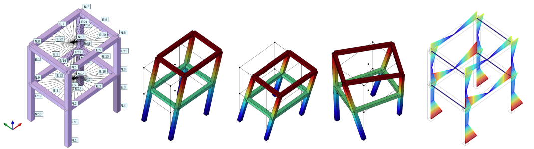
call the eigen Command to extract 7 modes of vibration
call the modalProperties Command to generate the report with modal properties
call the responseSpectrumAnalysis Command to compute the modal displacements and section forces * in a first example the responseSpectrumAnalysis Command is called for all modes. Results are obtained from a recorder after the analysis. * in a second example the responseSpectrumAnalysis Command is called in a for-loop mode-by-mode. Results are obtained within the for-loop usin the eleResponse
do a CQC modal combination
responseSpectrumAnalysisExample.py (Python).Code Developed by: Massimo Petracca at ASDEA Software, Italy