3.1.6.4. Drucker Prager Material

Code Developed by: Peter Mackenzie-Helnwein and Pedro Arduino at U.Washington.

This command is used to construct an multi dimensional material object that has a Drucker-Prager yield criterion.

nDMaterial DruckerPrager $matTag $k $G $sigmaY $rho $rhoBar $Kinf $Ko $delta1 $delta2 $H $theta $density <$atmPressure>

Argument	Type	Description
$matTag	float	integer tag identifying material
$k	float	bulk modulus
$G	float	shear modulus
$sigmaY	float	yield stress
$rho	float	frictional strength parameter
$rhoBar	float	controls evolution of plastic volume change: 0 ≤ $rhoBar ≤ $rho
$Kinf	float	nonlinear isotropic strain hardening parameter: $Kinf ≥ 0
$Ko	float	nonlinear isotropic strain hardening parameter: $Ko ≥ 0
$delta1	float	nonlinear isotropic strain hardening parameter: $delta1 ≥ 0
$delta2	float	tension softening parameter: $delta2 ≥ 0
$H	float	linear strain hardening parameter: $H ≥ 0
$theta	float	controls relative proportions of isotropic and kinematic hardening: 0 ≤ $theta ≤ 1
$density	float	mass density of the material
<$atmPressure>	float	optional atmospheric pressure for update of elastic bulk and shear moduli (default = 101 kPa)

Note

The material formulations for the Drucker-Prager object are “ThreeDimensional” and “PlaneStrain”

The yield condition for the Drucker-Prager model can be expressed as

\[f\left(\mathbf{\sigma}, q^{iso}, \mathbf{q}^{kin}\right) = \left\| \mathbf{s} + \mathbf{q}^{kin} \right\| + \rho I_1 + \sqrt{\frac{2}{3}} q^{iso} - \sqrt{\frac{2}{3}} \sigma_Y^{} \leq 0\]

in which

\[\mathbf{s} = \mathrm{dev} (\mathbf{\sigma}) = \mathbf{\sigma} - \frac{1}{3} I_1 \mathbf{1}\]

is the deviatoric stress tensor,

\[I_1 = \mathrm{tr}(\mathbf{\sigma})\]

is the first invariant of the stress tensor, and the parameters .. math::rho_{}^{}</math> and .. math::sigma_Y^{}</math> are positive material constants.

The isotropic hardening stress is defined as

\[q^{iso} = \theta H \alpha^{iso} + (K_{\infty} - K_o) \exp(-\delta_1 \alpha^{iso})\]

The kinematic hardening stress (or back-stress) is defined as

\[\mathbf{q}^{kin} = -(1 - \theta) \frac{2}{3} H \mathbb{I}^{dev} : \mathbf{\alpha}^{kin}\]

The yield condition for the tension cutoff yield surface is defined as

\[f_2(\mathbf{\sigma}, q^{ten}) = I_1 + q^{ten} \leq 0\]

where

\[q^{ten} = T_o \exp(-\delta_2^{} \alpha^{ten})\]

and

\[T_o = \sqrt{\frac{2}{3}} \frac{\sigma_Y}{\rho}\]

Further, general, information on theory for the Drucker-Prager yield criterion can be found at wikipedia here

Note

The valid queries to the Drucker-Prager material when creating an ElementRecorder are ‘strain’ and ‘stress’ (as with all nDmaterial) as well as ‘state’. The query ‘state’ records a vector of state variables during a particular analysis. The columns of this vector are as follows. (Note: If the option ‘-time’ is included in the creation of the recorder, the first column will be the time variable for each recorded point and the columns below are shifted accordingly.)

Column 1 - First invariant of the stress tensor, \(I_1 = \mathrm{tr}(\mathbf{\sigma})\). Column 2 - The following tensor norm, \(\left\| \mathbf{s} + \mathbf{q}^{kin} \right\| `, where .. math::\mathbf{s}\) is the deviatoric stress tensor and \(\mathbf{q}^{kin}\) is the back-stress tensor. Column 3 - First invariant of the plastic strain tensor, \(\mathrm{tr}(\mathbf{\varepsilon}^p) `. Column 4 - Norm of the deviatoric plastic strain tensor, :math:\)left| mathbf{e}^p right| `.

The Drucker-Prager strength parameters \(\rho ` and :math:\)sigma_Y ` can be related to the Mohr-Coulomb friction angle, \(\phi `, and cohesive intercept, :math:`c\), by evaluating the yield surfaces in a deviatoric plane as described by Chen and Saleeb (1994). By relating the two yield surfaces in triaxial compression, the following expressions are determined

\[\rho = \frac{2 \sqrt{2} \sin \phi}{\sqrt{3} (3 - \sin \phi)}\]

\[\sigma_Y = \frac{6 c \cos \phi}{\sqrt{2} (3 - \sin \phi)}\]

[Drucker-Prager1952]

Drucker, D. C. and Prager, W., “Soil mechanics and plastic analysis for limit design.” Quarterly of Applied Mathematics, vol. 10, no. 2, pp. 157–165, 1952.

[Chen-Saleeb1994]

Chen, W. F. and Saleeb, A. F., Constitutive Equations for Engineering Materials Volume I: Elasticity and Modeling. Elsevier Science B.V., Amsterdam, 1994.

Example

This example provides the input file and corresponding results for a confined triaxial compression (CTC) test using a single 8-node brick element and the Drucker-Prager constitutive model. A schematic representation of this test is shown below, (a) depicts the application of hydrostatic pressure, and (b) depicts the application of the deviator stress. Also shown is the stress path resulting from this test plotted on the meridian plane. As shown, the element is loaded until failure, at which point the model can no longer converge, as this is a stress-controlled analysis.

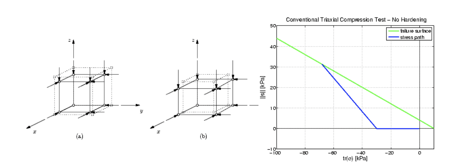
Fig. 3.1.6.1 Drucker Prager Example

#########################################################
##
# File is generated for the purposes of testing the#
#Drucker-Prager model --> conventional triaxial #
# compression test#
##
#   Created:  03.16.2009 CRM#
#   Updated:  12.02.2011 CRM#
##
# ---> Basic units used are kN and meters#
##
#########################################################

#-------------------------------------------------------
# create the modelBuilder and build the model
#-------------------------------------------------------
wipe

model BasicBuilder -ndm 3 -ndf 3

#--create the nodes
node 11.00.00.0
node 21.01.00.0
node 3 0.01.00.0
node 40.00.00.0
node 51.00.01.0
node 6 1.01.01.0
node 7 0.01.01.0
node 8 0.00.01.0

#--triaxial test boundary conditions
fix 1 0 1 1
fix 2 0 0 1
fix 31 0 1
fix 4 1 1 1
fix 50 1 0
fix 6 0 0 0
fix 71 0 0
fix 8 1 1 0

#--define material parameters for the model
#---bulk modulus
set k       27777.78
#---shear modulus
set G       9259.26
#---yield stress
set sigY    5.0
#---failure surface and associativity
set rho     0.398
set rhoBar  0.398
#---isotropic hardening
set Kinf    0.0
set Ko     0.0
set delta1  0.0
#---kinematic hardening
set H     0.0
set theta   1.0
#---tension softening
set delta2  0.0
#---mass density
        set mDen    1.7

#--material models
#   type         tag  k   G   sigY   rho   rhoBar   Kinf   Ko   delta1   delta2   H   theta   density 
nDMaterial DruckerPrager 2    $k  $G  $sigY  $rho  $rhoBar  $Kinf  $Ko  $delta1  $delta2  $H  $theta  $mDen

#--create the element
#type tag  nodesmatID  bforce1  bforce2  bforce3
element stdBrick 1    1 2 3 4 5 6 7 8   2      0.0      0.0      0.0

puts "model Built..."

#-------------------------------------------------------
# create the recorders
#-------------------------------------------------------
set step 0.1

# record nodal displacements
recorder Node -file displacements1.out -time -dT $step -nodeRange 1 8 -dof 1 2 3 disp

# record the element stress, strain, and state at one of the Gauss points
recorder Element -ele 1 -time -file stress1.out  -dT $step  material 2 stress
recorder Element -ele 1 -time -file strain1.out  -dT $step  material 2 strain
recorder Element -ele 1 -time -file state1.out   -dT $step  material 2 state

puts "recorders set..."

#-------------------------------------------------------
# create the loading
#-------------------------------------------------------

#--pressure magnitude
set p 10.0
set pNode [expr -$p/4] 

#--loading object for hydrostatic pressure
pattern Plain 1 {Series -time {0 10 100} -values {0 1 1} -factor 1} { 
    load 1  $pNode 0.00.0
    load 2  $pNode$pNode0.0
    load 3  0.0$pNode  0.0
    load 5  $pNode  0.00.0
    load 6  $pNode$pNode0.0
    load 7 0.0$pNode0.0
}

#--loading object deviator stress
pattern Plain 2 {Series -time {0 10 100} -values {0 1 5} -factor 1} { 
    load 5  0.00.0$pNode
    load 6  0.00.0$pNode
    load 7  0.00.0$pNode
    load 8  0.00.0$pNode
}

#-------------------------------------------------------
# create the analysis
#-------------------------------------------------------

integrator LoadControl 0.1
numberer RCM
system SparseGeneral
constraints Transformation
test NormDispIncr 1e-5 10 1
algorithm Newton
analysis Static

puts "starting the hydrostatic analysis..."
set startT [clock seconds]
analyze 1000

set endT [clock seconds]
puts "triaxial shear application finished..."
puts "loading analysis execution time: [expr $endT-$startT] seconds."

wipe