3.1.5.25. DowelType Timber Joint Material

This command is used to construct a uniaxial force-displacement or moment-rotation model which simulates the hysteresis of a dowel-type timber joint, including nails, screws, and bolts, etc. The model has the following features:

1. The envelope can be specified with any of the following models: (1) exponential, (2) cubic Bezier, and (3) piece-wise linear, by providing a flag before the defining parameters.

2. The envelopes can be defined either symmetric or asymmetric. Asymmetric envelopes can be defined by providing two sets of envelope parameters.

3. It is defined by the unloading line, pinching line, and reloading line, connected by Bezier curves to achieve a smooth stiffness transition.

4. It considers the varying of force intercept in the pinching part, defined according to the loading history.

5. It considers the degradation of unloading stiffness, pinching stiffness, and reloading stiffness, and defines the stiffness as an exponential function of either the maximum displacement to yield displacement ratio, or the secant stiffness to initial stiffness ratio.

6. It considers energy related degradation by using a energy-related damage index to amplify the maximum displacement as the reloading target point. The envelope curve is not changed during loading.

7. It considers the smooth transition of stiffness when the loading path goes from the pinching path directly to the envelope curve.

8. This model can simulate the behavior of joints with asymmetric layout, joints close to edges and restraints, joint groups with steel plates, joints with initial low-stiffness sliding range, etc.

The command to create a DowelType joint model has three variations, corresponding to different types of envelope curves.

(1) Use exponential envelope

uniaxialMaterial DowelType $matTag $Fi $Kp $Ru $c $beta $gamma $eta $Dy $alpha_p $alpha_u $alpha_r -exponential $K0 $R1 $F0 $Dc $Kd <$Du> <$K0N $R1N $F0N $DcN $KdN <$DuN>>

(2) Use Bezier envelope

uniaxialMaterial DowelType $matTag $Fi $Kp $Ru $c $beta $gamma $eta $Dy $alpha_p $alpha_u $alpha_r -bezier $Db1 $Fb1 $Db2 $Fb2 $Dc $Fc $Kd <$Du> <$Db1N $Fb1N $Db2N $Fb2N $DcN $FcN $KdN <$DuN>>

(3) Use piecewise envelope

uniaxialMaterial DowelType $matTag $Fi $Kp $Ru $c $beta $gamma $eta $Dy $alpha_p $alpha_u $alpha_r -piecewise $D1 $F1 $D2 $F2 $D3 $F3 <$D4 $F4 ...>

Universal parameters

Argument	Type	Description
$matTag	integer	Integer tag identifying material.
$Fi	float	Pinching line force intercept.
$Kp	float	Stiffness of the pinching line.
$Ru	float	Unloading stiffness to initial stiffness ratio.
$c	float	Hysteresis curvature factor. Curvature increases when c is larger. (0 <= $c < 2)
$beta	float	An amplification factor of the maximum displacement to account for maximum displacement based reloading stiffness and strength degradation. ( $beta >= 1 )
$gamma	float	A factor related to the energy-based damage index to account for energy based reloading stiffness and strength degradation. ( $gamma >= 1 )
$eta	float	A factor related to the extent that the force intercept varies with the maximum displacement. ( $eta >= 1 )
$Dy	float	Apparent yielding displacement.
$alpha_p	float	Stiffness degradation factor for pinching line.
$alpha_u	float	Stiffness degradation factor for unloading line.
$alpha_r	float	Stiffness degradation factor for reloading line.

Exponential envelope parameters

Argument	Type	Description
$K0	float	Initial stiffness.
$R1	float	Stiffness for the asymptotes of the envelope to initial stiffness ratio.
$F0	float	Envelope asymptotes force intercept.
$Dc	float	Cap displacement of the envelope.
$Kd	float	Absolute descending stiffness.
$Du	float	Ultimate displacement. By default the displacement intercept of the descending path is used.

Bezier envelope parameters

Argument	Type	Description
$Db1	float	The displacement of the first controlling point of the Bezier curve.
$Fb1	float	The force of the first controlling point of the Bezier curve.
$Db2	float	The displacement of the second controlling point of the Bezier curve.
$Fb2	float	The force of the second controlling point of the Bezier curve.
$Dc	float	Cap displacement of the envelope.
$Fc	float	Cap force of the envelope.
$Kd	float	Absolute descending stiffness.
$Du	float	Ultimate displacement. By default the displacement intercept of the descending path is used.

Piecewise envelope parameters

Argument	Type	Description
$D1	float	Displacement of the 1st piecewise linear envelope curve interpolation point.
$F1	float	Force of the 1st piecewise linear envelope curve interpolation point.
$D2	float	Displacement of the 2nd piecewise linear envelope curve interpolation point.
$F2	float	Force of the 2nd piecewise linear envelope curve interpolation point.
$D3	float	Displacement of the 3rd piecewise linear envelope curve interpolation point.
$F3	float	Force of the 3rd piecewise linear envelope curve interpolation point.

Note

1. The envelope curves can be either symmetric or asymmetric. Terms with a suffix N represents the definition for the negative part. If they are not provided, the envelope is symmetric.

2. The number of the interpolation points for the piecewise envelope curve should be not less than 3, and not larger than 20 (for a single side). If none of the displacements is negative, a symmetric envelope will be created. Otherwise, an asymmetric envelope will be created. It is better to sort the displacement from small to large. The origin point (0, 0) should not be included in the definition.

Envelope curves

The envelope curves are illustrated in the following figure. Only the positive part is illustrated.

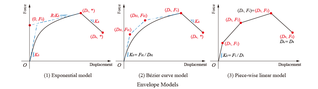
The expression of the exponential envelope curve is

\[\begin{split}F_{env}(D) = \begin{cases}(F_0+R_1 K_0 D)\left[ 1-\exp\left(\frac{-K_0 D}{F_0}\right) \right], & 0\leq D \leq D_c \\ F_c - K_d (D-D_c), & D_c < D \leq D_u \\ 0, & D > D_u \end{cases}\end{split}\]

where \(F_c\) is the force of the cap point. It can be calculated by

\[F_c = \left(F_0 + R_1 K_0 D_c \right) \left[1 - \exp\left(\frac{-K_0 D_c}{F_0}\right)\right]\]

and \(D_u\) is the ultimate displacement. Force after this displacement is set to zero. The default value is

\[D_u = \frac{F_c}{K_d} + D_c\]

The expression of the Bezier envelope curve for the ascending part is

\[\begin{split}\begin{cases}D_{env}(t) = 3t(1-t)^2 D_{b1} + 3t^2(1-t)D_{b2} + t^3D_c, & 0 \leq t \leq 1 \\ F_{env}(t) = 3t(1-t)^2 F_{b1} + 3t^2(1-t)F_{b2} + t^3 F_c, & 0 \leq t \leq 1\end{cases}\end{split}\]

Note

\((0, 0), (D_{b1}, F_{b1}), (D_{b2}, F_{b2}), (D_c, F_c)\) are the four controlling points of the cubic Bezier curve. \(0 < D_{b1} \leq D_{b2} < D_c\), and \(0 < F_{b1} \leq F_{b2} < F_c\)

After the cap point, the descending part is expressed as:

\[\begin{split}F_{env}(D) = \begin{cases} F_c - K_d (D-D_c), & D_c < D \leq D_u \\ 0, & D > D_u \end{cases}\end{split}\]

\(D_u\) is defined in the same manner as the exponential envelope.

The piecewise envelope connects all the definition points with straight lines. The ultimate displacement is the maximum (minimum for the negative part) displacement defined.

Hysteretic law

The hysteretic law is illustrated in the following figure. The hysteresis is independent from the envelope curve. Basically, the hysteretic curves are defined by three guiding lines: unloading line, pinching line, and reloading line. The lines define Bezier curves as shown in the figure.

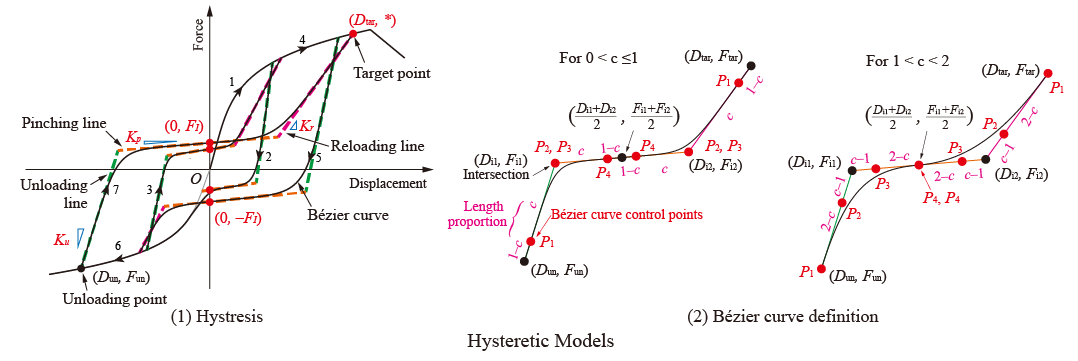
The pinching line passes a defined force intercept, expressed as:

\[\begin{split}F_{\mathrm{int}} = \begin{cases} \left(\frac{\left\lvert D_{m,s} \right\rvert}{D_y}\right) F_{I}, & \lvert D_{m,s} \rvert \leq D_y \\ F_{I}, & \lvert D_{m,s} \rvert > D_y \ \mathrm{and} \ \lvert F_{env}(D_{m,s}) \rvert \leq \lvert F_{env}(D_{y,s}) \rvert \\ F_{I} - \eta\left(F_{env}(D_{m,s})-F_{env}(D_{y,s})\right), & \lvert D_{m,s} \rvert > D_y \ \mathrm{and} \ \lvert F_{env}(D_{m,s}) \rvert > \lvert F_{env}(D_{y,s}) \rvert \end{cases}\end{split}\]

where \(D_{m,s}\) is the maximum displacement on the same side of the unloading point. \(D_{y,s}\) is the yielding displacement on the same side of the unloading point.

The reloading line passes a target point on the envelope curve, whose displacement is defined as:

\[D_{\mathrm{tar}} = \beta\gamma^{\lambda}D_{m,o}\]

\[\lambda = \frac{\Sigma E_{p,i} + \Sigma E_i}{E_f + \Sigma E_i}\]

where \(E_{p,i}\) is the energy dissipated in a primary half-cycle, \(E_i\) is the energy dissipated in the follower half-cycles, and \(E_f\) is the energy dissipated in a monotonic test to failure.

Note

The following figure is used to describe the same side and the opposite side:

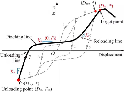
If unloading goes from large displacement to small displacement (i.e., right to left), \(D_{m,s}\) equals \(D_{max}\), and \(D_{m,o}\) equals \(D_{min}\). Otherwise, \(D_{m,s}\) equals \(D_{min}\), and \(D_{m,o}\) equals \(D_{max}\).

The stiffness of the three guiding lines are defined. In the definitions, degradation models are included. Two kinds of degradation models can be selected by specifying the sign of the related parameters. The stiffnesses are expressed as:

\[\begin{split}K_{\mathrm{pinching}} = \begin{cases} K_{p}, & \alpha_p \geq 0 \ \mathrm{and} \ D_m \leq D_y \\ K_{p}\left(\frac{D_y}{D_m}\right)^{\alpha_p}, & \alpha_p \geq 0 \ \mathrm{and} \ D_m > D_y \\ K_{p}\left(\frac{F_{env}(D_{m,s})}{D_{m,s}K_{0,s}}\right)^{\lvert\alpha_p\rvert}, & \alpha_p < 0 \end{cases}\end{split}\]

\[\begin{split}K_{\mathrm{unloading}} = \begin{cases} R_uK_{0,s}, & \alpha_u \geq 0 \ \mathrm{and} \ \lvert D_{m,s}\rvert \leq D_y \\ R_uK_{0,s} \left(\frac{D_y}{\lvert D_{m,s}\rvert}\right)^{\alpha_u}, & \alpha_u \geq 0 \ \mathrm{and} \ \lvert D_{m,s}\rvert > D_y \\ R_uK_{0,s} \left(\frac{F_{env}(D_{m,s})}{D_{m,s}K_{0,s}}\right)^{\lvert\alpha_u\rvert}, & \alpha_u < 0 \end{cases}\end{split}\]

\[\begin{split}K_{\mathrm{reloading}} = \begin{cases} K_{0,o}, & \alpha_r \geq 0 \ \mathrm{and} \ \lvert D_{m,o}\rvert \leq D_y \\ K_{0,o} \left(\frac{D_y}{\lvert D_{m,o}\rvert}\right)^{\alpha_r}, & \alpha_r \geq 0 \ \mathrm{and} \ \lvert D_{m,o}\rvert > D_y \\ K_{0,o} \left(\frac{F_{env}(D_{m,s})}{D_{m,s}K_{0,s}}\right)^{\lvert\alpha_r\rvert}, & \alpha_r < 0 \end{cases}\end{split}\]

where \(K_{0,s}\) and \(K_{0,o}\) are the stiffness on the same and opposite side of the unloading point, respectively. \(D_{m,s}\) is the maximum or minimum displacement on the same side of the unloading point. \(D_{m,o}\) is the maximum or minimum displacement on the opposite side of the unloading point.

There are also a few special scenarios, illustrated in the following figure:

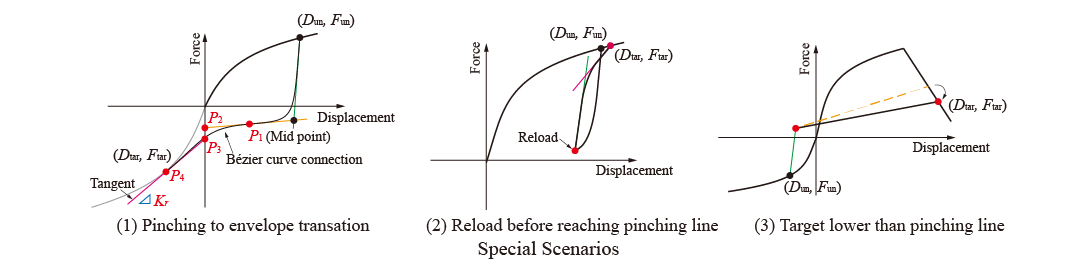
Special scenario 1 is the smooth transition from the pinching curve to the unloaded envelope curve.

Special scenario 2 is the case when reloading starts without reaching the pinching line.

Special scenario 3 is the case when large damage occurs. The hysteretic curve no longer reaches the pinching line.

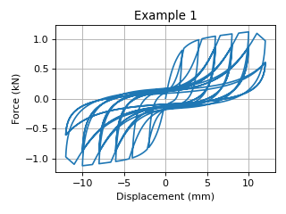
Example 1

The following command constructs a DowelType hysteretic model with tag 1. It simulates a nailed connection with symmetric exponential envelope curve.

1. Tcl Code

uniaxialMaterial DowelType 1 90 98.9 4.3 1.2 1.09 1.01 0.21 1.6 1.32 0 0.66 -exponential 823 0.02 955 10.7 123

2. Python Code

uniaxialMaterial('DowelType', 1, 90, 98.9, 4.3, 1.2, 1.09, 1.01, 0.21, 1.6, 1.32, 0, 0.66, '-exponential', 823, 0.02, 955, 10.7, 123)

The results of Example 1 is shown in the following figure:

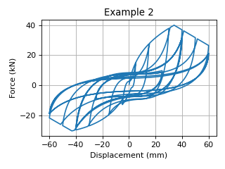
Example 2

The following command constructs a DowelType hysteretic model with tag 2. It simulates a CLT angle bracket connection under shear force. The yielding of the steel connector is considered within the single model. This example uses asymmetric Bezier curve as the envelope curve.

1. Tcl Code

uniaxialMaterial DowelType 2 445 170 3.8 1.3 1.03 1 0.34 3.2 0.92 0.03 -0.25 -bezier 3.2 19100 15 30500 34 40000 520 -5.3 -12800 -15.2 -25200 -43.1 -30400 510

2. Python Code

uniaxialMaterial('DowelType', 2, 445, 170, 3.8, 1.3, 1.03, 1, 0.34, 3.2, 0.92, 0.03, -0.25, '-bezier', 3.2, 19100, 15, 30500, 34, 40000, 520, -5.3, -12800, -15.2, -25200, -43.1, -30400, 510)

The results of Example 2 is shown in the following figure:

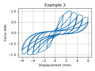
Example 3

The following command constructs a DowelType hysteretic model with tag 3. It simulates a nailed connection with asymmetric layout. It uses an asymmetric piecewise envelope curve.

1. Tcl Code

uniaxialMaterial DowelType 3 60 114.9 4.9 1.3 1.09 1 0.06 0.9 1.69 0.26 0.53 -piecewise 0.5 340 0.9 700 2.5 1030 10 300 -0.9 -600 -1.8 -800 -4.2 -1020 -10 -790

2. Python Code

uniaxialMaterial('DowelType', 3, 60, 114.9, 4.9, 1.3, 1.09, 1, 0.06, 0.9, 1.69, 0.26, 0.53, '-piecewise', 0.5, 340, 0.9, 700, 2.5, 1030, 10, 300, -0.9, -600, -1.8, -800, -4.2, -1020, -10, -790)

The results of Example 3 is shown in the following figure:

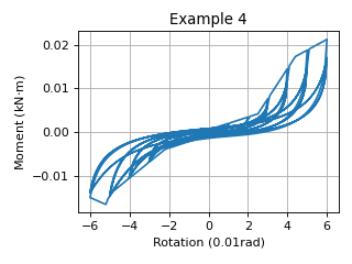
Example 4

The following command constructs a DowelType hysteretic model with tag 4. It simulates the moment-rotational behavior of a bolted connection with a small initial stiffness. It uses an asymmetric piecewise envelope curve.

1. Tcl Code

uniaxialMaterial DowelType 4 305 621.2 3.7 1.2 1.02 1 0.06 2.7 0.76 0.2 0 -piecewise 0.01 580 2.5 4200 4.4 17300 7 23700 10 16000 -0.1 -790 -2.2 -3900 -5 -14100 -5.2 -16500 -10 -7000

2. Python Code

uniaxialMaterial('DowelType', 4, 305, 621.2, 3.7, 1.2, 1.02, 1, 0.06, 2.7, 0.76, 0.2, 0, '-piecewise', 0.01, 580, 2.5, 4200, 4.4, 17300, 7, 23700, 10, 16000, -0.1, -790, -2.2, -3900, -5, -14100, -5.2, -16500, -10, -7000)

The results of Example 4 is shown in the following figure:

Code Developed by: Hanlin Dong (self@hanlindong.com) and Xijun Wang, Tongji University, China.

DongEtAl2021

Dong, H., He, M., Wang, X.*, Christopoulos, C., Li, Z., Shu, Z. (2021). “Development of a uniaxial hysteretic model for dowel-type timber joints in OpenSees.”, Construction and Building Materials, 288: 123112. DOI: https://doi.org/10.1016/j.conbuildmat.2021.123112