3.1.9.24. ASDAbsorbingBoundary Element (2D and 3D)

This command is used to construct an ASDAbsorbingBoundary2D or ASDAbsorbingBoundary3D object.

The ASDAbsorbingBoundary2D is a 4-node quadrilateral element, while the ASDAbsorbingBoundary3D is a 8-node hexaedron element.

This elements can be used as an extra layer at the boundaries of a soil domain to avoid wave reflections which typically arise with fixed boundaries.

element ASDAbsorbingBoundary2D $tag $n1 $n2 $n3 $n4 $G $v $rho $thickness $btype <-fx $tsxTag> <-fy $tsyTag>

element ASDAbsorbingBoundary3D $tag $n1 $n2 $n3 $n4 $n5 $n6 $n7 $n8 $G $v $rho $btype <-fx $tsxTag> <-fy $tsyTag> <-fz $tszTag>

Argument	Type	Description
$tag	integer	unique integer tag identifying element object.
$n1 $n2 $n3 $n4 $n5 $n6 $n7 $n8	4 (or 8) integer	the 4 (or 8) nodes defining the element.
$G	float	the shear modulus.
$v	float	the Poisson’s ratio.
$rho	float	the mass density.
$thickness	float	the thickness in 2D problems.
$btype	string	a string defining the boundary type. See Note 2
-fx	string	optional flag. if provided, the user should provide the velocity time-series along the X direction.
$tsxTag	integer	optional, mandatory if -fx is provided. the tag of the time-series along the X direction.
-fy	string	optional flag. if provided, the user should provide the velocity time-series along the Y direction.
$tsyTag	integer	optional, mandatory if -fy is provided. the tag of the time-series along the Y direction.
-fz	string	optional flag. if provided, the user should provide the velocity time-series along the Z direction.
$tszTag	integer	optional, mandatory if -fz is provided. the tag of the time-series along the Z direction.

3.1.9.24.1. Theory

When modelling a soil, only a portion of it is modelled, using artificial boundaries around it. Fixed conditions at these artificial boundaries are fine in static problems, but in dynamic problems they will reflect outgoing propagating waves. This problem can be avoided using a large portion of the model, which is impractical due to excessive computational efforts. Another solution is to adopt special boundary conditions which are able to absorb outgoing waves.

This element has been implemented following the work described in [Nielsen2006] for the 2D case, and properly extended for the 3D case. For a detailed theory explanation, please refer to [Nielsen2006] and the references therein.

In summary, this element can be seen as an assembly of many components:

• F: The Free-Field element, required to compute the free-field solution in parallel with the main model.

• D: The Lysmer-Kuhlemeyer dashpots, required to absorb outgoing waves.

• T: The boundary tractions transferred from the Free-Field to the Soil domain, required to impose the free-field solution to the boundaries of the main model.

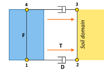
Fig. 3.1.9.29 Sketch of the absorbing (macro) element in 2D problems.

3.1.9.24.2. Usage Notes

Note 1

The element should have the standard node-numbering to ensure a proper positive jacobian.

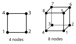
Fig. 3.1.9.30 Node numbering.

Note 2

The behavior of the element changes based on the side of the model it belongs to. The $btype argument defines the boundary type of the element. It is a string made of a combination of characters. Each character describes a side of the model:

• B = Bottom

• L = Left

• R = Right

• F = Front (only for 3D problems)

• K = Back (only for 3D problems)

For a 2D problem you can have the following valid combinations: B, L, R, BL, BR

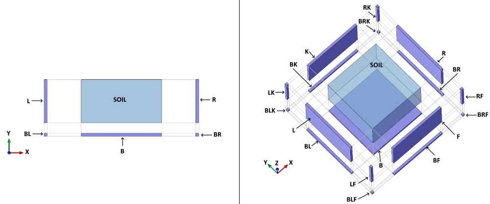
For a 3D problem you can have the following valid combinations: B, L, R, F, K, BL, BR, BF, BK, LF, LK, RF, RK, BLF, BLK, BRF, BRK

Fig. 3.1.9.31 Exploded-view: Boundary Type Codes for 2D (left) and 3D (right) problems.

Note 3

The element works in two stages.

In Stage 0, the element acts as a fix condition, suitable for the first gravity analysis. It stores the reactions and automatically converts them into applied boundary forces when switching from Stage 0 to Stage 1.

In Stage 1, the is converted into the real absorbing elements, and the reactions of the previous constraint element are applied as external forces.

The conversion from Stage 0 to Stage 1 can be done with the setParameter command (See Example)

Warning

• The boundary elements should be an extrusion of the sides of the main model along their outward normal vector.

• The vertical sides of the main model should have an outward normal vector that points either along the global (positive or negative) X direction or along the global (positive or negative) Y vector.

• The bottom side of the main model should have an outward normal vector that points in the negative global Z direction.

• In 3D models the sides L (left),R (right),F (front) and K (back) may have some natural distortion due to the topography. This is supported by the boundary element, but when the distortion along the Z direction is too large, the results can slightly deteriorate.

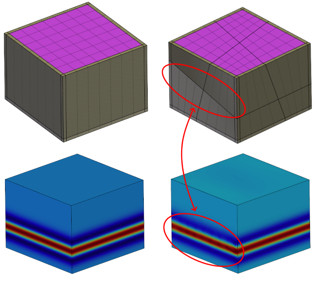
Fig. 3.1.9.32 Exploded-view: Effects of Z-distortion in 3D problems.

Example

1. Tcl Code

This is a small 2D example of a rectangular soil domain. The base input is a Ricker Wavelet.

With these boundary elements you should be able to 1) enforce the free-field solution on the soil domain and 2) absorb outgoing waves generated when the primary wave hits the free-surface.

This is the expected output: The blue line is the acceleration recorded at the base of the model. Point A and B represent respectively the wave entering the domain and the same wave exiting the domain after being reflected by the free surface. Their peak value should be exactly 1g. The purple line is the acceleration recorded at the top of the model (on the free surface). Point C represents the wave hitting the free-surface. Its peak value should be exactly 2g.

# ===================================================
# User parameters
# ===================================================
# material parameters
set E 3000000000.0
set poiss 0.3
set rho 2100.0
set thickness 1.0
set G [expr $E/(2.0*(1.0+$poiss))]
# domain size
set Lx 260.0
set Ly 140.0
# mesh size
set hx 10.0
set hy 1.0
# time increment
set dt 0.001
# predominant frequency of the Ricker Wavelet
set freq 10.0
# total duration of the dynamic analysis
set duration 1.0

# builder
model Basic -ndm 2 -ndf 2

# time series
# we want to apply a Ricker Wavelet with predominant frequency = 10 Hz.
# It should be applied as velocity
set pi [expr acos(-1.0)]
set wl [expr sqrt(3.0/2.0)/$pi/$freq*10.0]
set ndiv [expr int($wl/$dt)]
set dt [expr $wl/$ndiv.0]
set ts_vals {}
for {set i 0} {$i < $ndiv} {incr i} {
    set ix [expr $i.0*$dt-$wl/2.0]
    set iy [expr $ix*exp(-$pi*$pi*$freq*$freq*$ix*$ix)]
    lappend ts_vals $iy
}
set tsX 1
timeSeries Path $tsX -dt $dt -values $ts_vals  -factor 9.806

# material
set matTag 1
nDMaterial ElasticIsotropic $matTag $E $poiss $rho

# Define nodes on a regular grid with sizes hx-hy.
# For a more clear visualization we set the size of the absorbing elements larger.
# (note: the size of this element does not influence the results. The only constraint is that it
# should have a non-zero size!)
set ndivx [expr int($Lx/$hx) + 2]; # add 2 layers of absorbing elements (left and right)
set ndivy [expr int($Ly/$hy) + 1]; # add 1 layer of absorbing elements (bottom)
set abs_h [expr $hx*2.0]
for {set j 0} {$j <= $ndivy} {incr j} {
    if {$j == 0} {set y [expr -$abs_h]} else {set y [expr ($j-1) * $hy]}
    for {set i 0} {$i <= [expr $ndivx]} {incr i} {
        if {$i == 0} {set x [expr -$abs_h]} elseif {$i == [expr $ndivx]} {set x [expr $Lx+$abs_h]} else {set x [expr ($i-1) * $hx]}
        node [expr $j*($ndivx+1)+$i+1] [expr $x-$Lx/2.0] $y
    }
}

# Define elements.
# Save absorbing elements tags in a list
set abs_elements {}
for {set j 0} {$j < $ndivy} {incr j} {
    # Yflag
    if {$j == 0} {set Yflag "B"} else {set Yflag ""}
    for {set i 0} {$i < [expr $ndivx]} {incr i} {
        # Tags
        set Etag [expr $j*($ndivx)+$i+1]
        set N1 [expr $j*($ndivx+1)+$i+1]
        set N2 [expr $N1+1]
        set N4 [expr ($j+1)*($ndivx+1)+$i+1]
        set N3 [expr $N4+1]
        # Xflag
        if {$i == 0} {set Xflag "L"} elseif {$i == [expr $ndivx-1]} {set Xflag "R"} else {set Xflag ""}
        set btype "$Xflag$Yflag"
        if {$btype != ""} {
            # absorbing element
            lappend abs_elements $Etag
            if {$Yflag != ""} {
                # bottom element
                element ASDAbsorbingBoundary2D $Etag $N1 $N2 $N3 $N4 $G $poiss $rho $thickness $btype -fx $tsX
            } else {
                # vertical element
                element ASDAbsorbingBoundary2D $Etag $N1 $N2 $N3 $N4 $G $poiss $rho $thickness $btype
            }
        } else {
            # soil element
            element quad $Etag $N1 $N2 $N3 $N4 $thickness PlaneStrain $matTag 0.0 0.0 0.0 [expr -9.806*$rho]
        }
    }
}

# Static analysis (or quasti static)
# The absorbing boundaries now are in STAGE 0, so they act as constraints
constraints Transformation
numberer RCM
system UmfPack
test NormUnbalance 0.0001 10 1
algorithm Newton
integrator LoadControl 1.0
analysis Static
set ok [analyze 1]
if {$ok != 0} {
    error "Gravity analysis failed"
}
loadConst -time 0.0
wipeAnalysis

# update absorbing elements to STAGE 1 (absorbing)
setParameter -val 1 -ele {*}$abs_elements stage

# recorders
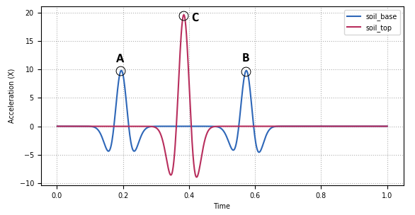
set soil_base [expr 1*($ndivx+1)+int($ndivx/2)+1]
set soil_top [expr $ndivy*($ndivx+1)+int($ndivx/2)+1]
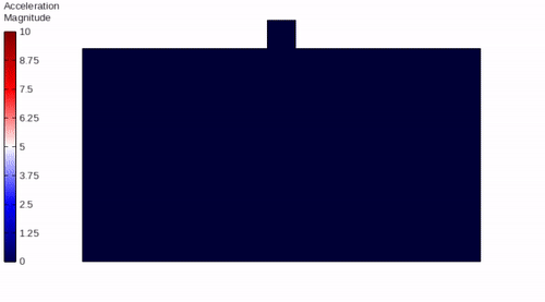
recorder Node -file "soil_base.txt" -time -node $soil_base -dof 1 accel
recorder Node -file "soil_top.txt" -time -node $soil_top -dof 1 accel

# Dynamic analysis
# The absorbing boundaries now are in STAGE 0, so they act as constraints
constraints Transformation
numberer RCM
system UmfPack
test NormUnbalance 0.0001 10 1
algorithm Newton
integrator TRBDF2
analysis Transient
set nsteps [expr int($duration/$dt)]
set dt [expr $duration/$nsteps.0]
set ok [analyze $nsteps $dt]
if {$ok != 0} {
    error "Dynamic analysis failed"
}

Code Developed by: Massimo Petracca at ASDEA Software, Italy.

Nielsen2006(1,2)

Nielsen, Andreas H. “Absorbing boundary conditions for seismic analysis in ABAQUS.” ABAQUS users’ conference. 2006.. (Link to article)